Jeffrey Baumgardner, Michael Mendillo, and Jody K. Wilson

Center for Space Physics

Boston University

725 Commonwealth Ave.

Boston, MA, 02215

Phone: 617-353-5258 (Baumgardner) -2629 (Mendillo) -7429 (Wilson)

Fax: 617-353-6463

E-mail: jkwilson@bu.edu

To appear in the Astronomical Journal, May 2000.

Abstract. We present an instrumentation plan for spectral imaging of Mercury's extended atmosphere. The approach depends upon simultaneous short-exposure images in white light and sodium, with the former used to select the frames for post-integration of the sodium images. The effects of atmospheric seeing are thus minimized by the combination of high-speed exposures and subsequent selective integration. The instrumentation to be used is a long slit imaging Echelle spectrometer equipped with an image slicer and an imaging photon detector. A test of the white light component of the technique has yielded a best-to-date image of a portion of Mercury's surface not photographed during the Mariner 10 mission.

The classic approach to imaging faint structures is to use the best available detector system with the longest exposures allowed by scattered light and atmospheric seeing conditions. If the target observed is stable in space and time, for large telescopes the factor that determines resolution is the degree of wave front distortion imposed by random atmospheric turbulence during the exposure time. The solution to the "seeing problem" most often used is to employ adaptive optics, i.e., a computer controlled deformation of the telescope optics to compensate for the effects of turbulence upon the image. A comprehensive treatment of such methods is given in Roggemann and Welsh (1996, and references therein).

Prior to the application of sophisticated technological solutions to atmospheric seeing problems, it was realized by virtually all expert naked-eye observers that instants of clarity occurred when telescopes performed at their theoretical "diffraction limited" abilities. Unfortunately, the detector in use (the human eye) did not have permanent storage capabilities, and so detailed drawings were made that merged the observer's observational skills with artistic abilities, psychological aspects of pattern recognition, and the unconscious desire to see new things. Yet, some of the more remarkable discoveries in astronomy were made precisely in this way, from Christiaan Huyghens' description of the rings of Saturn, to the discovery of Jupiter's red spot and the determination of Mars' rotation rate by J. D. Cassini. Less successful, but certainly more dramatic, were the renderings of features on Mars as glimpsed early in the 20th century. The "canals of Mars" described by Percival Lowell (1895, 1906,1908) in the US, and the larger-scale features portrayed by William ("eagle-eye") Dawes in the UK, have been treated by many authors (e.g., Holt, 1976; DeVorkin and Mendillo, 1979). Still, the core argument put forward by Lowell, namely, that the human eye can see in a split second what no camera can record, remains a challenge to the present day.

In this paper we outline an approach based upon the modern formulation of Lowell's grand idea, namely, high speed imaging coupled to a digital image storage system. The basis of the technique is described in Fried (1978) and in the excellent monograph by Roggemann and Welsh (1996). We chose as our test target the planet Mercury because adaptive optics approaches do not lend themselves easily to daytime observing and the Hubble Space Telescope is forbidden from observing an object so close to the Sun. In addition, preliminary results reported by Warell et al. (1998) show that albedo features on Mercury’s regolith can be seen in ground based broadband imaging.

An equally remarkable use of ground-based capabilities has been the spectroscopic detection of atmospheric gases (Na and K) by several groups (Potter and Morgan, 1985, 1986, 1987, 1990; Killen et al., 1990; Sprague et al., 1990, 1997a). Two-dimensional imaging of the surface's spectral signatures have also been successful at several wavelengths. Groundbased measurements in the infrared (McCord and Clark, 1979; Vilas et al., 1984; Sprague et al., 1997b) have been used to search for the chemical composition of Mercury’s surface, and airborne observations (Emery et al., 1999) for its thermal characteristics. Microwave observations (e.g., Mitchell and de Pater, 1994) are also used to explore surface composition.

The spectroscopic datasets published to date portray the spatial distribution of sodium just above Mercury’s limb. For more extended regions, there is one filtered two-dimensional image published (Potter and Morgan, 1997a). The comet-like appearance in that image has a sodium coma over a spatial scale (2-5 Mercury radii) larger than estimated by theory and simulation work (Smyth and Marconi, 1995) for a specific range of ejection speeds. In a more recent study, Potter et al. (1999) did not see such an extensive atmosphere. Thus, there is a real need for new and independent studies of the Hermean atmosphere. Identification of the size and shape of Mercury’s transient sodium atmosphere is, in itself, a central goal in studies of the sources and sinks of planetary exosphere’s (Morgan and Killen, 1997; Hunten and Sprague, 1997). Moreover, the relevance of such work is fundamental to our understanding of the similarly produced "surface-boundary-exosphere" of our Moon (Stern, 1999).

The linkage between remotely sensed surface characteristics (thermal and compositional), radar returns, and atmospheric signatures at Mercury (Sprague et al.,1998) awaits its final synthesis. In this paper, we describe a new approach for much needed data acquisition methods on Mercury's surface and atmosphere. Initial results are promising in that pilot studies in non-spectral mode have led to a new surface map of regions not viewed by the Mariner 10 spacecraft.

The application of monochromatic imaging techniques to Mercury presents some problems not encountered while observing other planetary targets. Since Mercury is always observed in twilight or daytime conditions, one needs to use a high (~1 Å) spectral resolution instrument to discriminate against the background continuum. In addition, Mercury’s radial velocity relative to the Sun and the Earth varies considerably with viewing geometry, requiring any spectral element to track the Doppler shifted wavelength of interest, or to have a large free spectral range to include this shift.

An interference filter can be tuned by heating or tilting, but it is difficult to produce filters with a 1 Å bandpass. Fabry-Perot interferometers have been used to observe the planets at high spectral resolution (e.g., Smyth et al., 1995), but unless a twin etalon system is used they do not have a large enough free spectral range to accommodate the large (3 Å) shift possible with a target such as Mercury. A high resolution grating spectrometer has the required spectral range and resolution but suffers from having a narrow slit that can only view a slice of a planet at any given time. To produce an image of an extended object such as a planet, the slit must be scanned across the disk, consequently loosing the time multiplex advantage of the filter or the etalon approaches mentioned above.

A new type of long slit échelle spectrograph has been developed at Boston University to study the terrestrial dayglow and aurora. These instruments, collectively called HiTIES, (High Throughput Imaging Echelle Spectrometer) share some common features: long (~50mm) input slits, reasonably fast (F/3.4 or F/10) collimators, and no cross dispersing elements. The image of the slit fills the spatial dimension of the detector. Interference filters are used to sort the various orders appearing on the detector. The medium resolution (R~10,000) variant of HiTIES uses a mosaic of filters near an image plane to select multiple lines of interest (Chakrabarti,1998). The high resolution (R~60,000) instrument uses interchangeable filters to select ~40Å regions around a given line of interest.

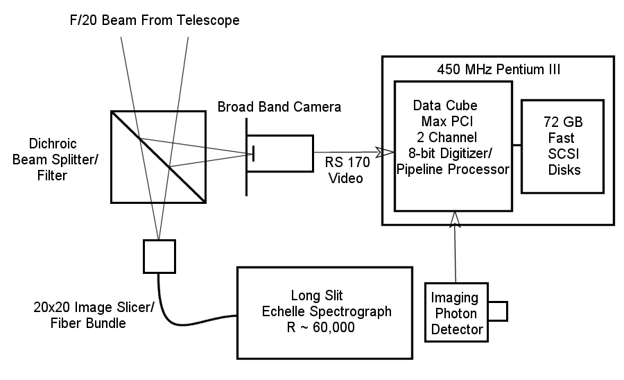
Figure 1. Schematic of the high definition imaging (HDI) system designed for integrated spectral imaging through a turbulent atmosphere.

A schematic of the monochromatic imaging system is shown in Figure 1. A pre-slit (i.e., pre-image slicer) viewer will be used to pick off ~10% of the beam for conventional broad band imaging to aid in pointing and, more importantly, to aid in subsequent selection and proper registration of images for co-adding. A later version of this pre-slit viewer will use a dichroic beam splitter that will allow ~95% of the out of band light to go to the viewer and ~80% of the on-band (HPFW ~50Å) light to go to the spectrograph. The procedure will be to record both the broad band image and the spectrograph image simultaneously at 60 images per second using a "real time" digitizer and a 72 Gigabyte disk array in a Pentium computer. The two cameras will be identical except that the camera on the spectrograph will be intensified, similar to those described in Baumgardner et al. (1993). The images from the spectrograph, after selecting a band pass and re-assembling a two-dimensional monochromatic image, will not have sufficient signal-to-noise in a single video field to determine quality of the seeing or precisely where the target is in the frame. The data from the broad band camera will be used to determine when the seeing is good and to find the optimum shift values. These values then will be used to align the re-constructed spectrograph images. We believe that this will be the first time this technique of combined beam-splitting and shifting-and-adding is used with an image slicer and a spectrograph to produce near-diffraction limited monochromatic images of planets.

Mercury was observed for about an hour on each of four days in August 1998. The observations typically began about one half hour before sunrise. After sunrise, the dome shutter and wind screen were used to shield the telescope optics and structure from direct sunlight. Once the sun was at more than ~5 degrees elevation, sunlight began heating the telescope structure, causing the focus to change and a noticeable degradation of the seeing. Table 1 lists the circumstances for the observations of Mercury made on August 27, 28, 29, and 30, 1998.

 Table 1: Mercury Observation Parameters for August 1999.

The individual images were saved as "tiles" in large (~ 650 Megabyte) files. Each file consists of ~100,000 individual, 1/60-second exposures. A series of tests was developed so that the computer can sort these images and reduce the number to a few hundred suitable for co-adding. The data from 29 August 1998 were chosen for further reduction.

After eliminating all fields where the entire image of Mercury was not visible (e.g., the image was cut off due to tracking errors), the remaining 219,000 images were characterized by a rotation angle (the camera was removed from the telescope several times during the observation period) and average sharpness or contrast. We used an image operator which effectively calculates the pixel-by-pixel contrast in an image:

Contrast at pixel(i,j) = | pixel(i,j) – pixel(i+1,j+1) | + | pixel(i+1,j) – pixel(i,j+1) |

Images were first smoothed to reduce pixel-to-pixel noise, the contrast operator was then applied, and the resulting images were squared to enhance small regions of high contrast (e.g., the limb) over large regions of low contrast (i.e., shades of gray across the crescent due to illumination). Finally we summed over the entire image to get a single number, or sharpness score, for each image. Figure 2 is a histogram of the sharpness scores for the 219,000 images used from August 29. Figure 2 also shows examples of images with low, medium, and high sharpness scores.

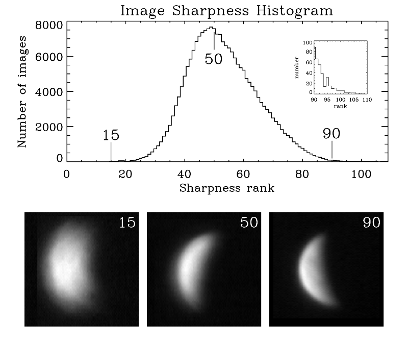
Figure 2. (Top) Distribution of approximately 219,000 images taken on 29 August 1999, sorted by their image sharpness as determined by the contrast algorithm rank. (Bottom) Sample images illustrating the effectiveness of contrast rank method of automated image selection for post integration.

The top 1000 images were re-ordered by considering their distortion or "rubber sheeting". Each image was compared to the average shape and then sorted by grouping the most similarly shaped images together. The top thirty images from each rotation were sub-pixel shifted by keying on one image in the group, and then co-added. The images were expanded by a factor of two in the y-direction to regain the correct aspect ratio before shifting and co-adding. The results of this procedure for the data taken on August 29 are shown in Figure 3, Panels A and B. For comparison, Panel C is the result of co-adding thirty consecutive video fields without shifting or selecting them for sharpness.

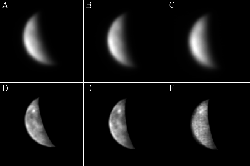
Figure 3. Combined and processed images of Mercury from August 29, 1999. In the interest of preserving as much detail as possible, these images have not been rotated from their original orientation on the camera. A and B: Averages of the best 30 images for each of two camera rotation angles. C: Average of 30 consecutive "typical" video images without shifting. D, E, and F: Maximum entropy deconvolution of images A, B, and C, respectively. To further enhance surface features, these images were divided by a function equal to the square-root of the cosine of the local solar zenith angle.

The images on Panels A, B and C of Figure 3 have improved signal-to-noise as compared to the single video fields shown in Figure 2. Panels D, E and F of Figure 3 are the same images as in Panels A, B and C, but have been sharpened using a maximum entropy method of de-convolving a point spread function (PSF) from the images. Since no star was observed simultaneously with Mercury, the limb profile of the co-added images was used to estimate the initial PSF. For these images, a Gaussian profile with a HPFW of 4 pixels was used (giving an effective resolution of ~250 km). Panels D and E show much improved surface detail whereas Panel F has a mottled appearance due to the reinforcement of fixed pattern noise on the CCD. (No suitable flat fields were available to correct the images before adding.) This fixed pattern noise is randomized in panels D and E because the component images are taken from different regions on the CCD. Figure 4 is the average of Panels D and E in Figure 3 and represents our overall portrayal of Mercury on this day. The rotation of both panels to portray a vertical terminator reduces pixel-to-pixel variations at the expense of smoothing contrast features seen more clearly on panels D and E.

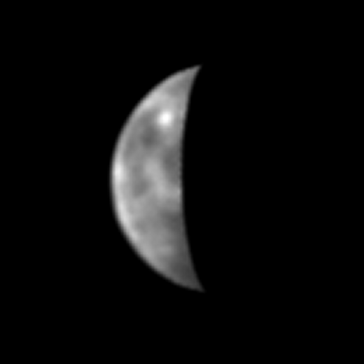
Figure 4. Combined average of the 60 best Mercury images of August 29, 1999, from Figure 3 (D and E).

To compare the radar and optical data, we map the image of Mercury from Figure 4 onto a Mercator projection, shown in Figure 5. Mariner 10 data provided by Hamilton (1999) is also included for reference. The left edge of the mapped region in Figure 5 is the limb and the right edge marks the terminator.

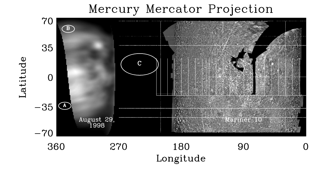
Figure 5. Mercator projections of Figure 4 and of Mariner 10 data (from Hamilton, 1999). Radar-bright spots A, B, and C are shown for comparison.

Radar maps of Mercury show the planet to be somewhat bland in reflective characteristics except at the poles and at three sites at mid-latitudes. One of these radar bright spots (termed "B" in Harmon (1997)) is within the longitude sector imaged, but there is no obvious relation to our albedo map, nor to the sodium seen near B by Sprague et al. (1998). The relationships between white light signatures, radar backscatter and reflectance spectroscopy are far from certain even in the Mariner imaged hemisphere.

Operationally, the digital recording system worked well, but the complete system will have to improve the through-put-to-disk by at least a factor of two since data will be obtained from two cameras simultaneously. Given that the narrow bandwidth (~1 Å) of the monochromatic imager will reduce the signal in the spectral image by three orders of magnitude, many more images will have to be coadded to achieve a sodium image approximately equivalent to the white light shown in Figure 4. To find this many images, the criteria for what constitutes a "good" image may have to be broadened.

The procedures described above will be applied to the less favorable data taken on August 27, 28, and 30. Some improvement in the images may be gained by segmenting the images into smaller regions (Dantowitz, 1998), recording a separate contrast number for each region, and then re-assembling complete images of Mercury.

Acknowledgements. The data used in this paper were obtained through a cooperative effort between the Center for Space Physics at Boston University and Ron Dantowitz of the Boston Museum of Science and Marek Kozubal. A companion paper appears in this issue describing the reduction of the analog (video tape) data of Mercury taken in August 1998 at Mt. Wilson. We are grateful to the Director and staff of the Mt. Wilson Observatory for their cooperation during these experiments. This work was supported by seed research funds made available via the Center for Space Physics at Boston University. We acknowedge the assistance of Mead Misic in the data analysis work, Clem Karl and Truong Nguyen for their helpful comments and discussion, and Supriya Chakrabarti for his support of the project. At Datacube, Inc., we acknowledge the assistance of Stan Karandanis and Chuan Zheng. Funding for instrumentation development has been provided by the Office of Naval Research.

Barlow, N. G., Ruth A. Allen, and F. Vilas, Mercurian impact craters: implications for polar ground ice, Icarus, 141, 194-204, 1999.

Baumgardner, J., B. Flynn, and M. Mendillo, Monochromatic imaging instrumentation for applications in aeronomy of the Earth and planets, Opt. Eng., 32(12), 1993.

Chakrabarti, S., Ground based spectroscopic studies of sunlit airglow and aurora, J. Atmosph. Solar Terr. Phys., 60, 1403-1424, 1998.

Dantowitz, R., Sharper Images Through Video, Sky and Telescope, 96, No. 2, 48-54, 1998.

DeVorkin, D. H., and M. Mendillo, The canals of Mars: A retrospective, Comm. J. Sci. Ed., 16, 4-19, 1979.

Fried, D. L., Probability of getting a lucky short-exposure image through turbulence, J. Opt. Soc. Am., 68, 1651-1658, 1978.

Goldstein, R. M., Radar observations of Mercury, Astron. J., 76, 1152-1154, 1971.

Hamilton, Calvin J., "http://planetscapes.com/solar/eng/mercmap.htm" in "Views of the Solar System, http://spaceart.com/solar/", 1999.

Harmon, J. K., Mercury Radar Studies and Lunar Comparisons, Adv. Space Res., 19, 1487-1496, 1997.

Harman, J. K., M. A. Slade, R. A. Velez, A. Crespo, M. J. Dryer, and J. M. Johnson, Radar mapping of Mercury’s polar anomalies, Nature, 369, 213-215, 1994.

Harmon, J. K., and M.A. Slade, On the Nature of the Major (Non-Polar) Radar Features in the Unimaged Hemisphere of Mercury, 1995 DPS Meeting.

Hoyt, W. G., Lowell and Mars, Univ. Ariz. Press, Tucson, 1976.

Killen, R. M., J. Benkhoff, and T. H. Morgan, Mercury’s polar caps and the generation of an OH exosphere, Icarus, 125, 195-211, 1997.

Killen, R. M., A. E. Potter, and T. H. Morgan, Spatial Distribution of Sodium Vapor in the Atmosphere of Mercury, Icarus, 85, 145-167, 1990.

Lowell, P., Mars, Longmans, Green and Co, London, 1885.

Lowell, P., Mars and Its Canals, The Macmillan Co., New York, 1906.

Lowell, P., Mars As the Abode of Life, The Macmillan Co., New York, 1908.

McCord, T. B., and R. N. Clark, The Mercury Soil: Presence of Fe²⁺, J. Geophys. Res., 84, 7664-7668, 1979.

Morgan, T. H., and R. M. Killen, A non-stoichiometric model of the composition of the atmospheres of Mercury and the Moon, Planet. Space Sci., 45, 81-94, 1997.

Moses, J. I., K. Rawlins, K. Zahnle, and L. Dones, External sources of water for Mercury's putative ice deposits, Icarus, 137, 197-221, 1999.

Potter, A. E., and T. H. Morgan, Discovery of sodium in the atmosphere of Mercury, Science, 229, 651-653, 1985.

Potter, A. E., and T. H. Morgan, Potassium in the atmosphere of Mercury, Icarus, 67, 336-340, 1986.

Potter, A. E., and T. H. Morgan, Variation of sodium on Mercury with solar radiation pressure, Icarus, 71, 472-477, 1987.

Potter, A. E., and T. H. Morgan, Evidence for magnetospheric effects on the sodium atmosphere of Mercury, Science, 248, 835-838, 1990.

Potter, A. E., and T. H. Morgan, Evidence for suprathermal sodium on Mercury, Adv. Space Res., 19, 1571-1576, 1997a.

Potter, A. E., and T. H. Morgan, Sodium and potassium atmospheres of Mercury, Planet. Space Sci., 45, 95-100, 1997b.

Potter, A. E., R. M. Killen, and T. H. Morgan, Rapid changes in the exosphere of Mercury, Planet. Space Sci., 47, 1441-1448, 1999.

Roggemann, M. C., and B. Welsh, Imaging Through Turbulence, CRC Press, Boca Raton (FL), 1996.

Slade, M. A., J. K. Harmon, P. J. Perillat, R. F. Jurgens, L. J. Harcke, High-Resolution Radar Imaging of Mercury’s North Pole with the Upgraded Arecibo Radar, Bull. Am. Astron. Soc., 31, 1132, 1999.

Smyth, W. H., M. R. Combi, F. L. Roesler, and F. Scherb, Observations and analysis of O(1D) and NH₂ line profiles for the coma of comet P/Halley, Astrophys. J., 440, 349-360, 1995.

Smyth, W. H., and M. L. Marconi, Theoretical overview and modeling of the sodium and potassium atmospheres of Mercury, Astrophys. J., 441, 839-864, 1995.

Sprague, A. L., D. M. Hunten, and K. Lodders, Sulfur at Mercury: Elemental at the poles and sulfides in the regolith, Icarus, 118, 211-215, 1995.

Sprague, A. L., R. W. H. Kozlowski, D. M. Hunten, Caloris Basin: An enhanced source for potassium in Mercury’s atmosphere, Science, 249, 1140-1143, 1990.

Sprague, A. L., R. W. H. Kozlowski, D. M. Hunten, N. M. Schneider, D. L. Domingue, W. K. Wells, W. Schmitt, and U. Fink, Distribution and abundance of sodium in Mercury’s atmosphere, 1985-1988, Icarus, 129, 506-527, 1997(a).

Sprague, A. L., D. B. Nash, F. C. Witteborn, and D. P. Cruikshank, Mercury’s feldspar connection: mid-IR measurements suggest Plagioclase, Adv. Space Res., 19, 1507-1510, 1997(b).

Sprague, A. L., W. J. Schmidt, and R. E. Hill, Mercury: Sodium atmospheric enhancements, radar bright spots, and visible surface features, Icarus, 135, 60-68, 1998.

Vasavada, A. R., D. A. Paige, and S. E. Wood, Near-surface temperatures on Mercury and the Moon and the stability of polar ice deposits, Icarus, 141, 179-193, 1999.

Vilas, F., M. A. Leake, and W. W. Mendell, The Dependence of Reflectance Spectra of Mercury on Surface Terrain, Icarus, 59, 60-68, 1984.

Warell , J., S. S. Limaye, and C.-I. Lagerkvist, Regolith albedo variegation on Mercury, Bull. Am. Astron. Soc., 30, 1111, 1998.